Long-Short Term Memory RNN
1 Why Simple RNN does not scale.
Consider a simple RNN given as:
\[ s_{i+1} = \sigma(As_i + Bx_i) \]
For simplicity, we assume a linear activation so \(s_{i+1} = As_i + Bx_i\).
Suppose we have a sequence \(\mathrm{seq} = \left<x_1, x_2, \dots, x_n\right>\). We can trace through the reduce operation:
\[ \begin{eqnarray} s_1 &=& As_0 + Bx_1 \\ s_2 &=& As_1 + Bx_2 = A^2s_0 + ABx_1 + Bx_2 \\ &\vdots& \\ s_n &=& A^ns_0 +\dots + Bx_n \end{eqnarray} \]
The loss function will be a function of the model parameter \(s_0\).
\[L(s_0, \dots) = f(A^ns_0 +\dots)\]
Thus:
\[ \frac{\partial L}{\partial s_0} = f'(\dots)\cdot A^n \propto A^n \]
1.1 Vanishing Gradient
If \(A\) has small elements, technically, \(\mathrm{eigvalue}(A) < 1\), then we have:
\[ \lim_{n\to\infty} \left(\frac{\partial L}{\partial s_0}\right) = 0 \]
Namely, inputs from the distant past do not affect the output.
1.2 Exploding Gradient
If \(A\) has large elements, technically, \(\mathrm{eigvalue}(A) > 1\), then we have:
\[ \lim_{n\to\infty} \left(\frac{\partial L}{\partial s_0}\right) \to \infty \]
Namely, inputs from the distant past completely determine the eventual output.
2 The Design of LSTM
We have two types of states:
Long-term memory, aka context: \[ C_{t}\in\mathbb{R}^d \]
Short-term memory, aka state: \[ h_{t}\in\mathbb{R}^d \]
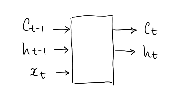
At each stage, we need to update both the context vector and the state vector:
\[ \left[\begin{array}{c} C_{t} \\ h_{t} \end{array}\right] = \mathbf{LSTM}(C_{t-1}, h_{t-1}, x_{t}) \]
Let’s define a linear layer with activation. This is commonly known as the fully connected layer.
\[ \mathbf{FC}(x) = Ax+b \]
where \(A\) and \(b\) are model parameters.
We will also be use the concatenation operator.
Suppose \(x\in\mathbb{R}^m\) and \(y\in\mathbb{R}^n\) be two vectors.
Then, we have:
\[ \left[\begin{array}{c} x \\ y \end{array}\right] \in\mathbb{R}^{m+n} \]
2.1 Updating context
The new context vector is a mixture of:
- part of the old context vector \(C_{t-1}\in\mathbb{R}^d\) to be remembered,
- part of the new vector \(\Delta C_{t}\in\mathbb{R}^d\),
- with the mixing coefficients \(f_t\in[0, 1]^d\) and \(i_t\in[0, 1]^d\).
\[ C_{t} = f_t* C_{t-1} + i_t*\Delta C_{t} \]
The values \(f_t\), \(i_t\) and \(\Delta C_{t}\) will be learned.
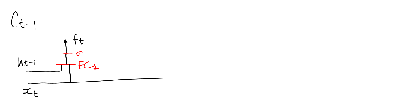
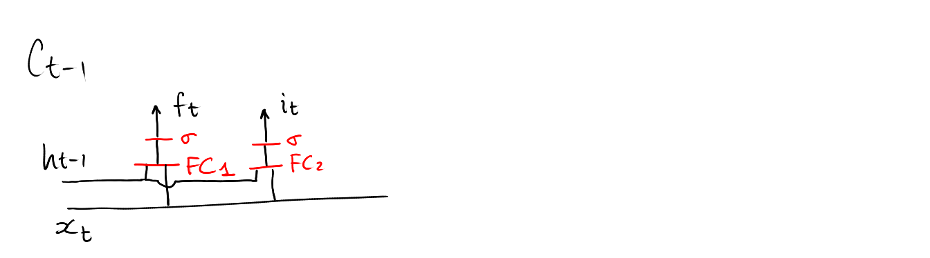
\[ f_t = \mathrm{sigmoid}\circ\mathbf{FC}_1\left( \left[\begin{array}{c} h_{t-1} \\ x_t \end{array}\right] \right) \in[0,1]^d \]
\[ i_t = \mathrm{sigmoid}\circ\mathbf{FC}_2\left( \left[\begin{array}{c} h_{t-1} \\ x_t \end{array}\right] \right) \in[0,1]^d \]
\[ \Delta C_t = \mathrm{tanh}\circ\mathbf{FC}_3\left( \left[\begin{array}{c} h_{t-1} \\ x_t \end{array}\right] \right) \in\mathbb{R}^d \]
2.2 Updating state
The new state is learned from the new context vector.
\[ h_t = o_t * \mathrm{tanh}(C_t) \]
where \(o_t\in[0, 1]^d\) is learned from:
\[ o_t = \mathrm{sigmoid}\circ\mathbf{FC_4}\left( \left[\begin{array}{c} h_{t-1} \\ x_t \end{array}\right] \right) \in[0,1]^d \]
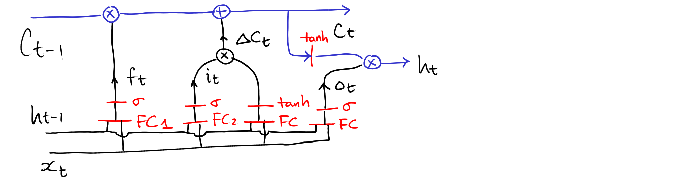
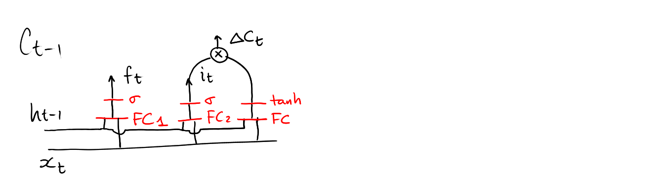
3 Network architecture of a single stage LSTM
Computing \(f_t\)
Computing \(i_t\)
Computing \(\Delta C_t\)
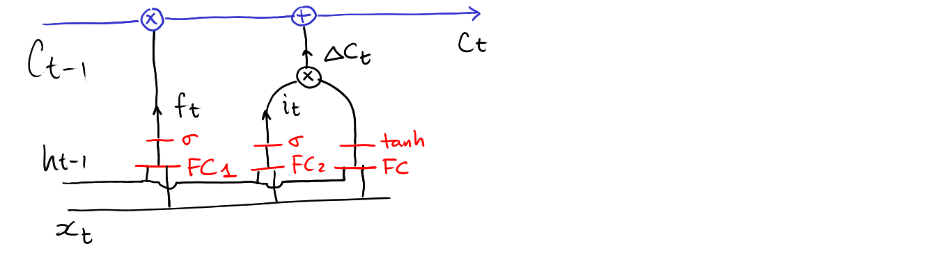
Computing \(C_t\)
Computing \(o_t\)
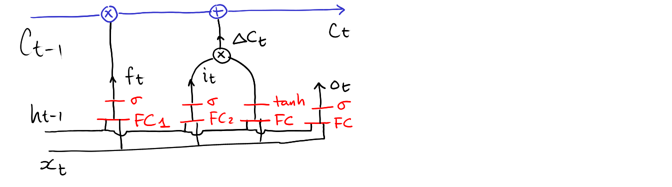
Computing \(h_t\)