import numpy as np
import matplotlib.pyplot as pyplot☑ Linear Algebra
1 Scalars
1.1 What are scalars?
- Value of \(\pi\)
- Grade for math
- Height of a person
- Birth year of Albert Einstein
- Color of the Canadian flag
- My favourite season of the year
1.2 Data types
- Float: \(\mathbb{R}\)
- Positive floats: \(\mathbb{R}^+\)
- Fraction: \([0, 1]\)
- Integer: \(\mathbb{N}\)
- Categorical: \(\{\mathrm{red}, \mathrm{green}, \mathrm{blue}\}\)
1.3 Different kinds of scalars
- Constant values
- Variables:
- Dependent
- Independent
- Unknown
1.4 Measuring closeness of scalars
Consider two scalars \(x\) and \(y\)
Similarity measure: \[ \mathrm{sim}(x, y) \in [-1, 1] \] \[ \mathrm{sim}(x, x) = 1 \]
Here is an example: \[ \mathrm{sim}(x, y) = \frac{\min(x, y)}{\max(x, y)} \]
Distance measure: \[ d(x, y) \in [0, \infty) \] \[ d(x, x) = 0 \] \[ \forall x, y, z,\ d(x, y) \leq d(x, z) + d(z, y) \quad \mathrm{triangular\ inequality} \]
Here is an example: \[ d(x, y) = |x - y| \]
Here is another example: \[ d(x, y) = (x - y)^2 \]
2 Vectors
2.1 Examples
Some examples of vectors:
Grades for math, english and biology: \[ x = \left[\begin{array}{c} g_\mathrm{math} \\ g_\mathrm{english} \\ g_\mathrm{biology} \end{array}\right] \in \mathbb{R}^3 \]
Person with height, weight, IQ and income. \[ x = \left[\begin{array}{c} \mathrm{height} \\ \mathrm{weight} \\ \mathrm{IQ} \\ \mathrm{income} \end{array}\right]\in\mathbb{R}^4 \]
2.2 Notation
An entry in a vector is a scalar.
\[ x = [x_1, x_2, x_3, \dots, x_n] \in \mathbb{R}^n \]
\[ x = \left[\begin{array}{c} x_1 \\ x_2 \\ x_3 \\ \vdots \\ x_n \end{array}\right]\in\mathbb{R}^n \]
Each entry \(x_i\in\mathbb{R}\).
2.2.1 Magnitudes of vectors
Let \(x\in\mathbb{R}^n\), its magnitude is given as:
\[ \|x\| = \sqrt{\sum_{i=1}^n x_i^2} \]
We usually express the magnitude squared:
\[ \|x\|^2 = \sum_{i=1}^n x_i^2 \]
Distance between two vectors can be expressed as a magnitude. \[ d(x,y) = \|x - y\| \]
2.2.2 Inner product
Consider two vectors that have the same dimensionality: \(x, y \in \mathbb{R}^n\).
Inner product
\[\left<x,y\right> = \sum_{i=1}^n x_i\cdot y_i\]
Magnitude as an inner product:
\[ \|x\|^2 = \left<x, x\right> \]
2.2.3 Measuring closeness: similarity
Consider two vectors that have the same dimensionality: \(x, y \in \mathbb{R}^n\)
We can measure the similarity of two vectors based on the angle between them.
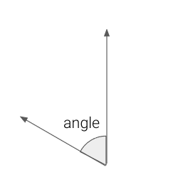
Note:
\[ \begin{eqnarray} \cos(\theta) &=& \frac{\sum_{i=1}^n x_iy_i}{\sqrt{\left(\sum_{i=1}^n x_i^2\right)\left(\sum_{i=1}^n y_i^2\right)}} \\ &=& \frac{\left<x, y\right>}{\|x\| \|y\|}\\ &\in& [-1, 1] \end{eqnarray} \]
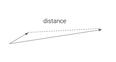
2.2.4 Measuring closeness: distance
\[ \begin{eqnarray} d(x, y) &=& \sqrt{\sum_{i=1}^n (x_i - y_i)^2} \\ &=& \|x - y\| \end{eqnarray} \]
3 Matrices
A matrix is a grid of scalars. A matrix has two axes: rows and columns.
\(A_{ij}\in\mathbb{R}\) is an entry where \(i\in[1, m]\) and \(j\in[1, n]\)
\(A\) is a matrix of shape \((m, n)\)
\(A\in\mathbb{R}^{m\times n}\)
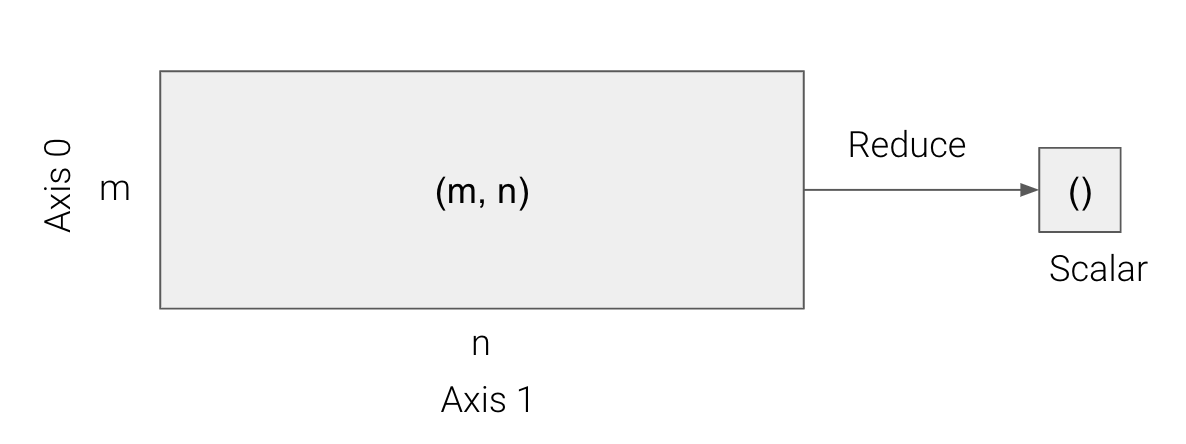
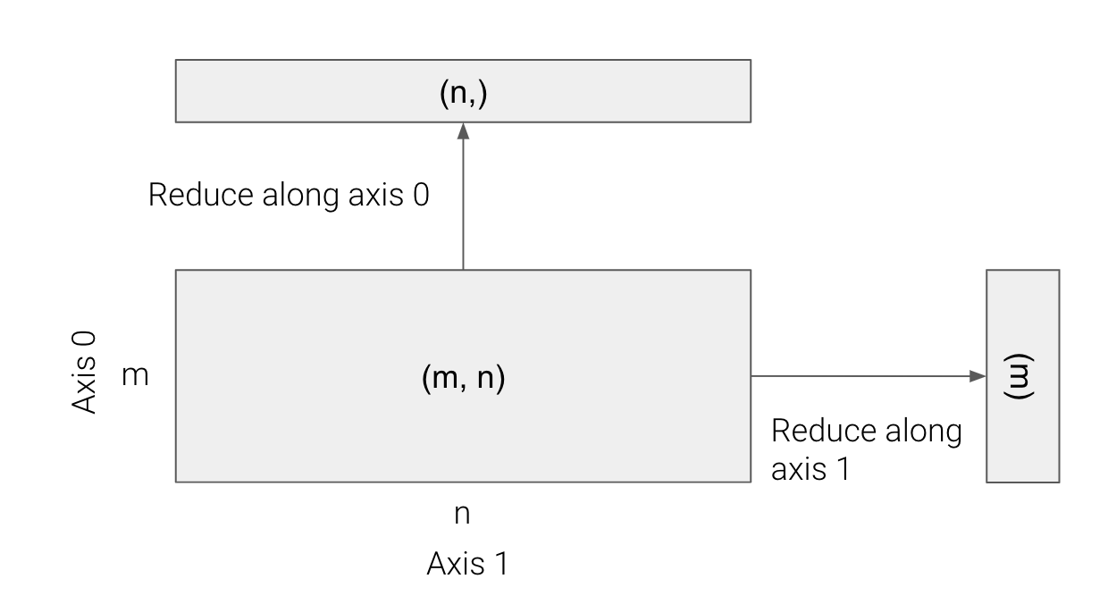
3.1 Reduction
Reduction functions are functions that map vectors or matrices to a scalar.
\[ h: A \mapsto v \]
Some examples are:
- Summation: \(h(A) = \sum_{i=1}^m\sum_{j=1}^n A_{ij}\)
- Mean
- Max / Min
3.2 Reducing along an axis
We can apply any reduction function along an axis. This results in a vector.
\[ h_\mathrm{axis=0} : \mathbb{R}^{m\times n} \to \mathbb{R}^n \]
\[ h_\mathrm{axis=0}(A)[j] = h(A[:,j]) \]
4 Transformations
4.1 A single vector
vector = np.array([1., 2.])

pyplot.scatter([vector[0]], [vector[1]], s=100)
pyplot.grid(True)
pyplot.xlim((-5, 5))
pyplot.ylim((-5, 5));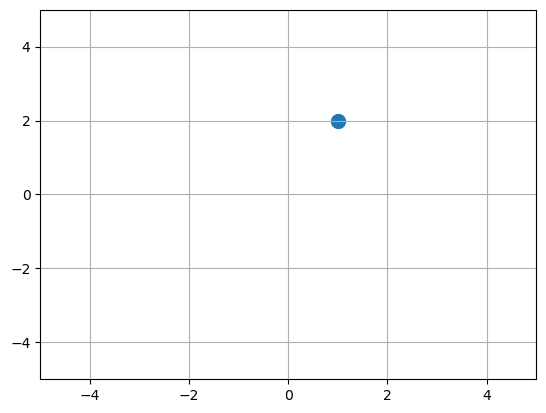
4.2 A collection of vectors
xs = np.random.normal(0, 1, size=(1000,))
ys = np.random.normal(0, 2, size=(1000,))

vectors = np.vstack([xs, ys])
vectors.shape
(2, 1000)Let’s plot them.
pyplot.figure(figsize=(6, 6))
pyplot.xlim((-10, 10))
pyplot.ylim((-10, 10))

pyplot.scatter(vectors[0, :], vectors[1, :], s=1);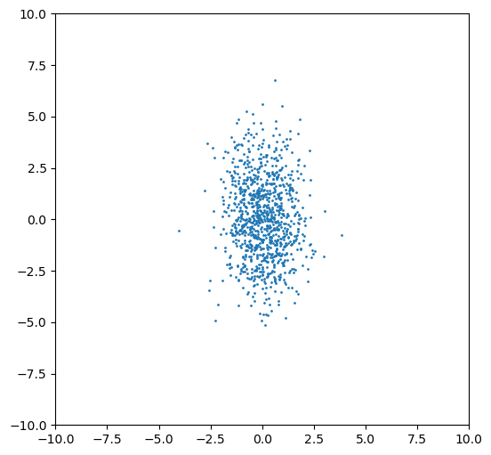
4.3 Scaling axes by matrices
Here is a scaling matrix:
- grows x-coordinates by 3
- shrinks y-coordinates by 1/3
M = np.array([
    [3, 0],
    [0, 1/3]
])

M.shape
(2, 2)We can apply the scaling to the vectors:
x = M @ vectors
x.shape
(2, 1000)Let’s see the effect of matrix multiplication when \(M\) is a scaling matrix.
pyplot.figure(figsize=(6, 6))
pyplot.xlim((-10, 10))
pyplot.ylim((-10, 10))

pyplot.scatter(vectors[0, :], vectors[1, :], s=1, color='gray');
pyplot.scatter(x[0, :], x[1, :], s=1, color='red');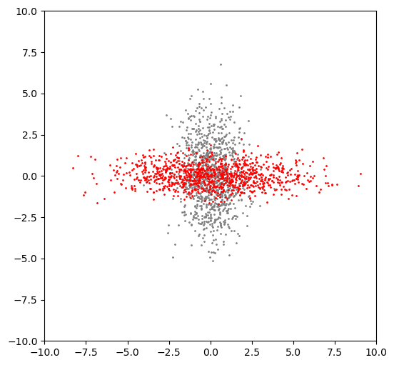
4.4 Rotational matrix
The general form of a rotational matrix is:
\[ R = \left[\begin{array}{cc} \cos(\theta) & \sin(\theta) \\ -\sin(\theta) & \cos(\theta) \end{array}\right] \] where \(\theta\) is the clockwise rotation angle.
theta = np.pi / 4        # 45 degrees

R = np.array([
    [np.cos(theta), np.sin(theta)],
    [-np.sin(theta), np.cos(theta)]
])

R.shape
(2, 2)We can apply the rotational matrix to the set of vectors.
x = R @ vectors
x.shape
(2, 1000)Let’s see the effect of matrix multiplication when \(R\) is a rotation matrix.
pyplot.figure(figsize=(6, 6))
pyplot.xlim((-10, 10))
pyplot.ylim((-10, 10))

pyplot.scatter(vectors[0, :], vectors[1, :], s=1, color='gray');
pyplot.scatter(x[0, :], x[1, :], s=1, color='red');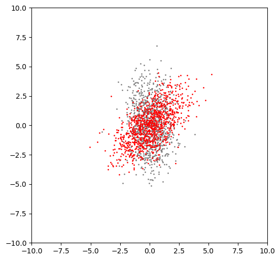
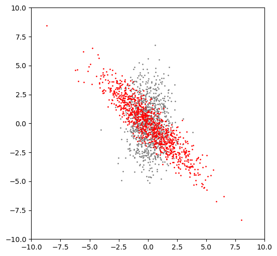
4.5 Compositional transformation
Here is the composition that performs rotation and then translation.
x = M @ R @ vectors
x.shape
(2, 1000)pyplot.figure(figsize=(6, 6))
pyplot.xlim((-10, 10))
pyplot.ylim((-10, 10))
pyplot.scatter(vectors[0, :], vectors[1, :], s=1, color='gray');
pyplot.scatter(x[0, :], x[1, :], s=1, color='red');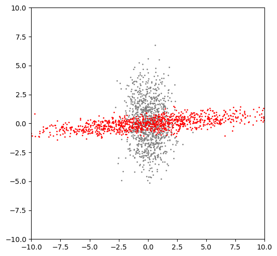
Now, consider the composition that performs translation followed by rotation.
x = R @ M @ vectors
x.shape
(2, 1000)pyplot.figure(figsize=(6, 6))
pyplot.xlim((-10, 10))
pyplot.ylim((-10, 10))
pyplot.scatter(vectors[0, :], vectors[1, :], s=1, color='gray');
pyplot.scatter(x[0, :], x[1, :], s=1, color='red');