import torch
from torch.utils.data import Dataset, IterableDataset☑ Training
1 Mathematical overview
1.1 Input-output spaces
\(\mathcal{X}\) is the input space. This will be some type of mathematical representation of the underlying data including text, image, audio, databases, etc.
\(\mathcal{T}\) is the target space.
1.2 Observed data
We make observations which consists of pairs of inputs and their respective outputs.
- A single observation is \((x, t) \in\mathcal{X}\times\mathcal{T}\). We also call \((x,y)\) a sample.
- Collectively, a set of observations is called a dataset \[D = \{(x_i, t_i): 1\leq x\leq N\}\]
1.3 Functional model
We speculate a functional relationship between \(\mathcal{X}\) and \(\mathcal{Y}\). Namely, there exists some function that describes the mapping from \(x_i\) to \(y_i\) in the observations.
\[ f^* : \mathcal{X}\to\mathcal{Y} \] such that \[ y_i = f^* (x_i) \]
In general, the target space \(\mathcal{T}\) and the output space \(\mathcal{Y}\) are not the same, but equivalent. Namely they are easily comparable. We will discuss the connection between \(\mathcal{T}\) and \(\mathcal{Y}\) when we talk about loss functions.
1.4 Function template and parameters
In order to find such function \(f^*\), we first fix a template for such function:
- \(f_\theta\) is a function template. Namely, it is a family functions that share the same structure, but differ by their own parameters \(\theta\).
- \(\theta\) is one or more tensors that is part of the function definition. We call \(\theta\) the model parameter.
Thus, we speculate that the functional model \(f^*\) has the same structure as \(f_\theta\), but has a specific model parameter.
\[ f^* = f_{\theta^*} \]
1.5 Loss functions
A loss function allows us to connect the target space of the observations and the output space of the functional model.
\[\mathrm{loss} : \mathcal{Y}\times\mathcal{T}\to\mathbb{R} \]
It maps a pair \((y, t)\) to a scalar value that determines the degree of match between \(y\) and \(t\). The smaller \(\mathrm{loss}(y, t)\) it is, the better the match \(y\) is with \(t\).
1.6 Model evaluation
A model \(f:\mathcal{X}\to\mathcal{Y}\) can be evaluated with respect to a given dataset \(D\subseteq\mathcal{X}\times\mathcal{T}\) by a loss function \(\mathrm{loss}:\mathcal{Y}\times\mathcal{T}\to\mathbb{R}\).
\[ L(f, D) = \sum_{i\leq N} \mathrm{loss}(f(x_i), t_i)) \]
1.7 Parameter optimization
Given a function template \(f_\theta\) parameterized by \(\theta\), we can learn better and better model parameters using gradient based optimization that minimizes the loss value.
Define \[ L(\theta, D) = L(f_\theta, D) \]
The final functional model of \(D\) is \(f^* = f_{\theta^*}\) where
\[ \theta^* = \mathrm{argmin}\{L(\theta, D):\theta\in\mathrm{Parameter\ Space}\} \]
2 Training Data Pipeline
2.1 Gradient optimization
Let’s review the gradient based optimization.
Pseudo code for epoch based training
def train(
    parameters: List[Parameter],
    model: Function,
    loss_function: Function,
    training_data: Dataset,
    ...
):
    LOOP:
        loss = sum([
            loss_function(
                model(x, parameters),
                t
            ) for (x, t) in training_data)
        ])
        for p in parameters:
            p.zero_grad()
        loss.backward()
        for p in parameters:
            p.sub_(learning_rate * p.grad)
    END LOOP
Each loop is called an epoch which corresponds to a single pass of the entire training dataset.
The pseudo code is impracticel for several reasons.
- Summing over the entire dataset creates a huge computational graph, making
loss.backward()too costly. - The entire dataset may not fit into memory, so
losscannot be computed in memory.
2.2 Batch training
Batch training relies on two approaches:
- The parameter gradient can be estimated using a sample of the training data.
- Dataset can be partitioned into small samples known as batches.
Here is the pseudo code for batch training.
Batch training
def batch_train(
    parameters: List[Parameter],
    model: Function,
    loss_function: Function,
    training_data: Dataset,
):
    LOOP:
    |   for batch in load_batches_of(training_data):
    |   |   loss = sum([
    |   |       loss_function(
    |   |           model(x, parameters),
    |   |           t,
    |   |       ) for (x, t) in batch
    |   |   ])
    |   |   for p in parameters:
    |   |       p.zero_grad()
    |   |   loss.backward()
    |   |   for p in parameters:
    |   |       p.sub_(learning_rate * p.grad)
    END LOOP
2.3 Data loader
In the body of batch_train, the load_batches_of(training_data) function call is commonly known as a data loader.
A data loader is responsible for:
- Generating small batches of samples from the large dataset. Each batch has the same size, known as the batch size.
- Grouping samples of a batch into a single tensor for the inputs, and a single tensor for the targets.
- Optionally shuffle the samples for better estimation of the parameter gradients.
3 Torch abstraction of datasets
Let’s see how batch training is done in PyTorch.
3.1 Index based dataset
We can define a custom dataset based on Dataset class. We must implement several methods:
__init__(...)initializes the dataset.__len__(self)computes the total number of samples in the dataset.__getitem__(self, index)returns the sample at positionindex.
Note, this assumes that we can access all of the samples directly.
#
# A simple curve fitting example: y = 3x + sin(6x) + 1, for x in [0, 1]
#

class MyCurve(Dataset):
    def __init__(self, num_points):
        self.xs = torch.linspace(0, 1, num_points)
    def __len__(self):
        return self.xs.shape[0]
    def __getitem__(self, i):
        x = self.xs[i]
        y = 3*x + torch.sin(6*x) + 1
        return x, y
Let’s try out the dataset.
ds = MyCurve(100)
print("len =", len(ds))
print(ds[42])
len = 100
(tensor(0.4242), tensor(2.8342))3.2 Iterator based datasets
- What if the dataset is so large that it does not fit into memory?
- What if we are downloading the dataset over the network (e.g. Twitter feeds), so that we cannot easily access the observation at a particular index?
We want to use an iterator based dataset.
class StreamedCurve(IterableDataset):
    def __init__(self, start, end, delta):
        self.start = torch.tensor(start, dtype=torch.float)
        self.end = torch.tensor(end, dtype=torch.float)
        self.delta = torch.tensor(delta, dtype=torch.float)
    def __iter__(self):
        def f(x):
            return 3*x + torch.sin(6*x) + 1
        x = self.start
        while x < self.end:
            yield x, f(x)
            x = x + self.delta
Let’s try to get some samples from the streamed curve.
ds = StreamedCurve(0, 2, 0.1)
iterator = iter(ds)
next(iterator), next(iterator), next(iterator)
((tensor(0.), tensor(1.)),
(tensor(0.1000), tensor(1.8646)),
(tensor(0.2000), tensor(2.5320)))4 Torch abstraction of data loading
from torch.utils.data import DataLoaderds = StreamedCurve(0, 2, 0.01)
dataloader = DataLoader(ds, batch_size=32)batch = next(iter(dataloader))
batch[tensor([0.0000, 0.0100, 0.0200, 0.0300, 0.0400, 0.0500, 0.0600, 0.0700, 0.0800,
0.0900, 0.1000, 0.1100, 0.1200, 0.1300, 0.1400, 0.1500, 0.1600, 0.1700,
0.1800, 0.1900, 0.2000, 0.2100, 0.2200, 0.2300, 0.2400, 0.2500, 0.2600,
0.2700, 0.2800, 0.2900, 0.3000, 0.3100]),
tensor([1.0000, 1.0900, 1.1797, 1.2690, 1.3577, 1.4455, 1.5323, 1.6178, 1.7018,
1.7841, 1.8646, 1.9431, 2.0194, 2.0933, 2.1646, 2.2333, 2.2992, 2.3621,
2.4220, 2.4786, 2.5320, 2.5821, 2.6287, 2.6719, 2.7115, 2.7475, 2.7799,
2.8088, 2.8340, 2.8557, 2.8738, 2.8885])]import matplotlib.pyplot as pyplot
iterator = iter(dataloader)
(x1, y1) = next(iterator)
(x2, y2) = next(iterator)
(x3, y3) = next(iterator)
pyplot.plot(
x1, y1, '--',
x2, y2, '-',
x3, y3, '-.');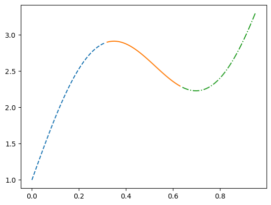
ds = MyCurve(100)
dataloader = DataLoader(ds, batch_size=32, shuffle=True)

iterator = iter(dataloader)
(x1, y1) = next(iterator)
(x2, y2) = next(iterator)
(x3, y3) = next(iterator)

pyplot.plot(
    x1, y1, '--',
    x2, y2, '-',
    x3, y3, '-.');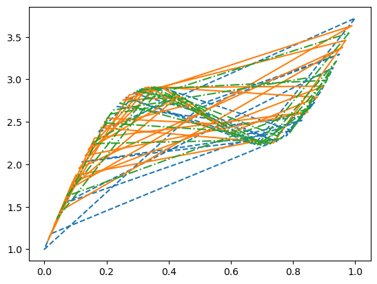
5 Torch abstraction of model
import torch.nn as nn
import torch.nn.functional as F
class MyModel(nn.Module):
def __init__(self):
super().__init__()
self.layer1 = nn.Linear(1, 16)
self.layer2 = nn.Linear(16, 1)
def forward(
self,
x, # (batch,)
):
x = x[:, None] # (batch, 1)
x = self.layer1(x) # (batch, 16)
x = F.sigmoid(x) # (batch, 16)
x = self.layer2(x) # (batch, 1)
x = x.squeeze(1) # (batch,)
return xdataloader = DataLoader(MyCurve(100), batch_size=32, shuffle=True)
(x, target) = next(iter(dataloader))
x.shape, target.shape(torch.Size([32]), torch.Size([32]))f = MyModel()
y = f(x)
y.shapetorch.Size([32])#
# Check the loss
#
with torch.no_grad():
loss = F.mse_loss(y, target)
losstensor(8.1953)6 Batch Training with Lightning
6.1 LightningModule = Module + Loss + Optimizer
from lightning.pytorch import LightningModule
import torch.optim as optim
class MyLtModule(LightningModule):
def __init__(self):
super().__init__()
self.layer1 = nn.Linear(1, 16)
self.layer2 = nn.Linear(16, 1)
def forward(
self,
x, # (batch,)
):
x = x[:, None] # (batch, 1)
x = self.layer1(x) # (batch, 16)
x = F.sigmoid(x) # (batch, 16)
x = self.layer2(x) # (batch, 1)
x = x.squeeze(1) # (batch,)
return x
def loss(self, y, target):
return F.mse_loss(y, target)
def training_step(self, batch, batch_index):
"Returns the loss tensor"
(x, target) = batch
loss = self.loss(self.forward(x), target)
self.log('loss', loss, prog_bar=True)
return loss
def configure_optimizers(self):
"Returns an optimizer"
return optim.Adam(self.parameters())A lightning module packages multiple useful features into a single class.
f = MyLtModule()
batch = next(iter(dataloader))

with torch.no_grad():
    batch_loss_0 = f.training_step(batch, 0)

batch_loss_0tensor(7.8143)6.2 Trainer
from lightning.pytorch import Trainertraining_dataloader = DataLoader(MyCurve(1024), batch_size=32, shuffle=True)
f = MyLtModule()trainer = Trainer(max_epochs=10)GPU available: False, used: False
TPU available: False, using: 0 TPU cores
IPU available: False, using: 0 IPUs
HPU available: False, using: 0 HPUstrainer.fit(f, training_dataloader)
  | Name   | Type   | Params
----------------------------------
0 | layer1 | Linear | 32
1 | layer2 | Linear | 17
----------------------------------
49        Trainable params
0         Non-trainable params
49        Total params
0.000     Total estimated model params size (MB)
`Trainer.fit` stopped: `max_epochs=10` reached.
with torch.no_grad():
y = f.forward(batch[0])
batch_loss_1 = f.loss(y, batch[1])
batch_loss_1tensor(0.3247)6.3 Logging
from lightning.pytorch.loggers import CSVLoggerlogger = CSVLogger('lightning_logs', name='my_lt_module')
trainer = Trainer(logger=logger, max_epochs=30)GPU available: False, used: False
TPU available: False, using: 0 TPU cores
IPU available: False, using: 0 IPUs
HPU available: False, using: 0 HPUsf = MyLtModule()
trainer.fit(f, train_dataloaders=training_dataloader)
  | Name   | Type   | Params
----------------------------------
0 | layer1 | Linear | 32
1 | layer2 | Linear | 17
----------------------------------
49        Trainable params
0         Non-trainable params
49        Total params
0.000     Total estimated model params size (MB)
`Trainer.fit` stopped: `max_epochs=30` reached.
import pandas as pd
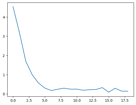
df = pd.read_csv('./lightning_logs/my_lt_module/version_1/metrics.csv')
df.head()| loss | epoch | step | |
|---|---|---|---|
| 0 | 4.534048 | 1 | 49 |
| 1 | 3.198307 | 3 | 99 |
| 2 | 1.698596 | 4 | 149 |
| 3 | 0.999312 | 6 | 199 |
| 4 | 0.559942 | 7 | 249 |
df['loss'].plot.line();