import numpy as np
import matplotlib.pyplot as pyplot☑ Lines and Planes
1 Projection between vectors
Let \(u\in\mathbb{R}^n\) be a vector.
Its normal vector is denoted as \(\hat u\), defined as the vector in the same direction as \(u\), but with length 1.
\[ \hat u = \frac{u}{\|u\|} \]
Given two vectors \(u, v\in\mathbb{R}^n\), the projection of \(u\) on \(v\) is the vector that is the closest to \(u\) in the direction of \(v\).
\[ \mathbf{proj}(u, v) = \left< u, \hat v\right>\hat v \]
u = np.array([2., -1.])
v = np.array([1, 1])

v_hat = v / np.linalg.norm(v)
proj = (u @ v_hat) * v_hat
proj.shape(2,)pyplot.figure(figsize=(6,6))
pyplot.plot([0, u[0]], [0, u[1]])
pyplot.plot([0, v[0]], [0, v[1]], color='gray')
pyplot.plot([proj[0], u[0]], [proj[1], u[1]], color='red')
pyplot.plot([0, proj[0]], [0, proj[1]], color='red')
pyplot.scatter([proj[0]], [proj[1]], color='red', s=30);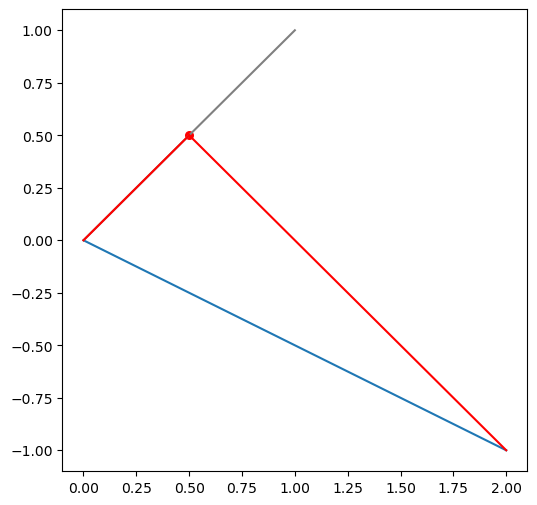
2 Lines
2.1 Line through the origin
Lines are defined as a collection of vectors in \(\mathbb{R}^n\) such that all the points defined by the vectors are on a straight line.
\[ L_u = \{ c\cdot u: c\in\mathbb{R} \} \]
u = np.array([1, 1])
c = np.linspace(-5, 5, 50)

L = c[:, None] @ u[None, :]

L.shape
(50, 2)pyplot.scatter(L[:, 0], L[:, 1], s=20, color='gray', alpha=0.5)
pyplot.scatter([0], [0], s=50, color='red')
pyplot.grid(True);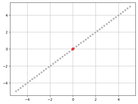
2.2 Line not through the origin
These are also called lines with bias.
\[ L_{u,b} = \{c\cdot u + b: c\in\mathbb{R}\} \]
u = np.array([1, 1])
b = np.array([2, -5])

L = c[:, None] * u[None, :] + b
L.shape
(50, 2)pyplot.scatter(L[:, 0], L[:, 1], s=20, color='gray', alpha=0.5)
pyplot.scatter([0], [0], s=50, color='red')
pyplot.scatter([b[0]], [b[1]], s=50, color='blue')
pyplot.grid(True);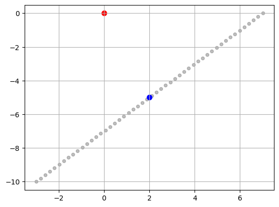
3 Planes
3.1 Planes through the origin given by two directional vectors
\[ P_{u,v} = \{a\cdot u + b\cdot v: a, b\in\mathbb{R}\} \]
u = np.array([-0.3, -0.4, 0.8])
v = np.array([0.7, -0.67, 0])

a = np.linspace(-10, 10, 50)
b = np.linspace(-10, 10, 50)
L1 = a[:, None] @ u[None, :]
L2 = b[:, None] @ v[None, :]

grid = L1[:, None, :] + L2[None, :, :]
P = grid.reshape(-1, 3)
P.shape
(2500, 3)fig = pyplot.figure(figsize=(6, 6))
ax = fig.add_subplot(projection='3d')
ax.set_xlim(-5, 5)
ax.set_ylim(-5, 5)
ax.set_zlim(-5, 5)
ax.scatter(P[:, 0], P[:, 1], P[:, 2], s=5, alpha=0.5, color='gray');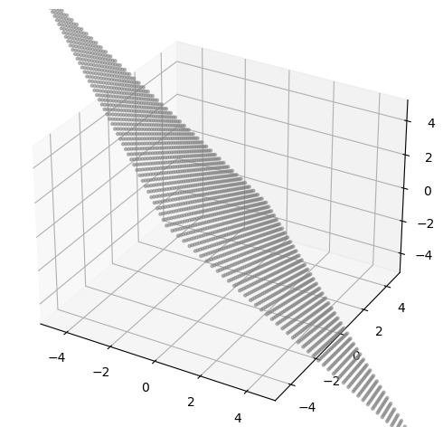
3.2 Plane through the origin defined by one normal vector
\[ P = \{x\in\mathbb{R}^n: \left< x,w\right> = 0\} \] where \(w\in\mathbb{R}^n\).
The two formulations are in fact equivalent.
Find the first direction vector
Let \(z\in\mathbb{R}^n\) be any vector. We observe that \(z\) can be decomposed into a component \(z_1\) that is in the direction of \(w\), and a normal component that is perpendicular to \(w\).
\[ z_1 = \mathbf{proj}(z, w) \]
Thus,
\[ z_2 = z - z_1 = z - \mathbf{proj}(z, w) \]
\(z_2\) is guaranteed to be perpendicular to \(w\).
Find the second direction vector
Recall the result from linear algebra: the cross product of two vectors is a vector that is perpendicular to both vectors. https://en.wikipedia.org/wiki/Cross_product
The second directional vector can be found as:
\[ z_2\times w = (z - \mathbf{proj}(z, w))\times w \]
# Define a normal vector to a plane in 3D

w = np.array([2.0, 3.0, 4.0])
w
array([2., 3., 4.])#
# Let's compute the first direction vector of the plane
#
# start with a random vector
z = np.array([1, 1, 1])
# compute projection
w_norm = w / np.sqrt(w @ w)
z_proj = (z @ w_norm) * w_norm
z1 = z - z_proj
z1array([ 0.37931034, 0.06896552, -0.24137931])#
# Verify that z1 is a direction vector
#
z1 @ w-1.1102230246251565e-16#
# Let's compute the second direction vector of the plane using cross product
#
z2 = np.cross(w, z1)
z2array([-1., 2., -1.])#
# Verify z2
#
z2 @ w4.440892098500626e-16u = z1
v = z2
a = np.linspace(-10, 10, 50)
b = np.linspace(-10, 10, 50)
L1 = a[:, None] @ u[None, :]
L2 = b[:, None] @ v[None, :]
grid = L1[:, None, :] + L2[None, :, :]
P = grid.reshape(-1, 3)
fig = pyplot.figure(figsize=(6, 6))
ax = fig.add_subplot(projection='3d')
ax.set_xlim(-5, 5)
ax.set_ylim(-5, 5)
ax.set_zlim(-5, 5)
ax.scatter(P[:, 0], P[:, 1], P[:, 2], s=5, alpha=0.3, color='gray');
#
# Plot w as well
#
ax.plot([0, w[0]], [0, w[1]], [0, w[2]]);
ax.scatter([w[0]], [w[1]], [w[2]], color='red');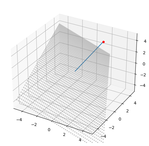
Normal vector is preferred
Planes are a central recurring character in machine learning. In most cases, we will present planes by their normal vectors.
3.3 Projection onto a plane
We assume that the plane \(P_w\) goes through the origin.
Consider a general vector \(v\in\mathbb{R}^n\). Its projection on \(P\) is defined as the point \(x^*\in P\) such that \(x^*\) is the closest to $v.
\[ \mathbf{proj}(v, P) = v - \mathbf{proj}(v, w) \]
Can you prove the formula geometrically?
3.4 Planes with bias
A plane does not always have to go through the origin. Planes that do not contain the origin are called planes with bias.
\[ P_{w, b} = \{x\in\mathbb{R}^n: \left<x, w\right> + b = 0\} \] where \(b\in\mathbb{R}\).
The constant \(b\) is called the bias.
Find a point on the plane
Consider the point in \(\mathbb{R}^n\) in the form of: \[x = c\cdot w\] where \(c\in\mathbb{R}\) is just a scalar.
We want to choose \(c\) such that \(x\in P_{w,b}\).
\[ \begin{eqnarray} x\in P_{w,b} &\implies& \left<x,w\right> + b = 0 \\ &\implies& \left<cw,w\right> + b = 0 \\ &\implies& c\|w\|^2 = -b \\ &\implies& c = -\frac{b}{\|w\|^2} \end{eqnarray} \]
Thus: \[ -\frac{b}{\|w\|^2}w \in P_{w,b} \]
3.5 Projection on planes with bias
We can work out projections on planes with bias using coordinate transformations.
Start with:
- \(v\in\mathbb{R}^n\)
- \(P_{w,b}\subseteq\mathbb{R}^n\)
We define a coordinate transformation \(h: x\mapsto x' = x - (-b/\|w\|^2)w = x + \frac{b}{\|w\|^2}w\). Similarly, the inverse mapping is \(h^{-1}:x'\mapsto x=x'-\frac{b}{\|w\|^2}w\).
- \(v' = h(v)\)
- \(P' = h(P)\) is a plane without bias.
We can compute \(\mathbf{proj}(v', P')\), and then translate it back to the original coordinates:
\[ \mathbf{proj}(v, P) = h^{-1}(\mathbf{proj}(v', P')) \]
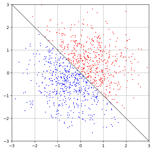
3.6 Planar separation
X = np.random.randn(1000, 2)

pyplot.figure(figsize=(6,6))
pyplot.xlim(-3, 3)
pyplot.ylim(-3, 3)
pyplot.grid(True)
pyplot.scatter(X[:, 0], X[:, 1], s=1);
pyplot.plot([-3, 3], [3, -3], color='gray');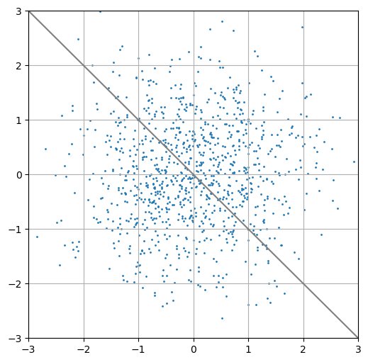
w = np.array([1, 1])

top_half = X @ w > 0
bottom_half = X @ w < 0

pyplot.figure(figsize=(6,6))
pyplot.xlim(-3, 3)
pyplot.ylim(-3, 3)
pyplot.grid(True)
pyplot.scatter(X[top_half, 0], X[top_half, 1], s=1, color='red')
pyplot.scatter(X[bottom_half, 0], X[bottom_half, 1], s=1, color='blue');
pyplot.plot([-3, 3], [3, -3], color='gray');