☐ Evaluation

import matplotlib.pyplot as pyplot
import pandas as pd
import numpy as np

1 Overfitting

import torch
import torch.nn as nn
import torch.nn.functional as F
import torch.optim as optim

1.1 Noisy data

To illustrate the danger of wielding the computational power freely to learn from data, let’s consider the following linear but noisy dataset.

\[ y = 2x + 1 + \mathrm{noise} \]

torch.manual_seed(0)
xs = torch.linspace(0, 1, 20)
target = 2 * xs + 1 + 0.3 * torch.randn(20);

pyplot.plot(xs, target, '--o');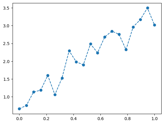

1.2 Learning from noisy data

class MLP(nn.Module):
    def __init__(self, hidden_dim, num_hidden_layers):
        super().__init__()
        self.layer1 = nn.Linear(1, hidden_dim)
        self.layers = nn.ModuleList([
            nn.Sequential(
                nn.Linear(hidden_dim, hidden_dim),
                nn.Sigmoid(),
            )
        ])
        self.layer_last = nn.Linear(hidden_dim, 1)
    def forward(
        self,
        x,    # (batch,)
    ):
        x = x[:, None]            # (batch, 1)
        x = self.layer1(x)        # (batch, hidden)
        for layer in self.layers:
            x = layer(x)
        x = self.layer_last(x)    # (batch, 1)
        x = x[:, 0]               # (batch,)
        return x

simple_model = MLP(2, 1)
optimizer = optim.Adam(simple_model.parameters())
num_epochs = 5000

from tqdm.notebook import trange
with trange(num_epochs) as progress:
    for epoch in progress:
        loss = F.mse_loss(simple_model(xs), target)
        optimizer.zero_grad()
        loss.backward()
        optimizer.step()
        loss = loss.detach().numpy()
        progress.display('loss:{:.2f}'.format(loss))

with torch.no_grad():
    output = simple_model(xs)
    loss = F.mse_loss(output, target)
loss

tensor(0.0642)

pyplot.plot(xs, target, 'o', xs, output);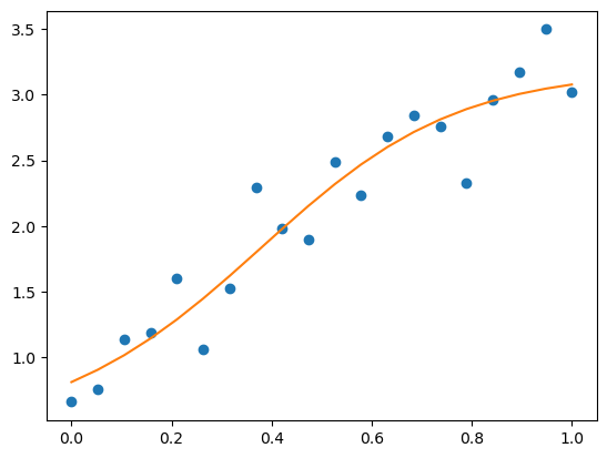

The simple_model has achieved good fit of the noisy data. Numerically, the loss function is 0.06.

1.3 Large models

large_model = MLP(hidden_dim=1024, num_hidden_layers=8)

optimizer = optim.Adam(large_model.parameters())
num_epochs = 5000

from tqdm.notebook import trange
with trange(num_epochs) as progress:
    for epoch in progress:
        loss = F.mse_loss(large_model(xs), target)
        optimizer.zero_grad()
        loss.backward()
        optimizer.step()
        loss = loss.detach().numpy()
        progress.display('loss:{:.2f}'.format(loss))

with torch.no_grad():
    output = large_model(xs)
    loss = F.mse_loss(output, target)
pyplot.plot(xs, target, 'o', xs, output)
loss

tensor(0.0016)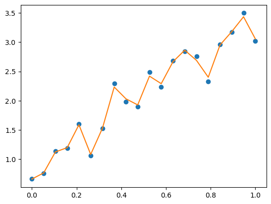

The large_model achieved a “better” loss value of 0.0016, but objectively, we would say that large_model has achieved a worse fit as it no longer follows the trend in the data, but rather following the noise of the data.

How do we justify that large_model is worse than the simple_model?

2 Validation

Validation is a technique to assess the quality of a model by holding out a portion of the available samples for evaluation. This is known as the validation dataset. In most cases, validation datasets are not used for training.

\[ D = D_\mathrm{train} \cup D_\mathrm{val} \]

torch.manual_seed(0)
xs_train = torch.linspace(0, 1, 20)
target_train = 2 * xs_train + 1 + 0.3 * torch.randn(20);

xs_val = torch.linspace(1, 1.8, 15)
target_val = 2 * xs_val + 1 + 0.3 * torch.randn(15);

pyplot.plot(xs_train, target_train, '--o', xs_val, target_val, 'o');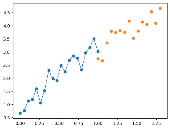

2.1 Valuation loss

The validation loss is defined as:

\[ L_\mathrm{val}(\theta, D_\mathrm{val}) \]

models = {
    'simple_model': simple_model,
    'large_model': large_model
}

losses = {
    'val_loss': [],
    'train_loss': [],
}
for (name, model) in models.items():
    with torch.no_grad():
        output = model(xs_val)
        losses['val_loss'].append(F.mse_loss(output, target_val).item())
        
        output = model(xs_train)
        losses['train_loss'].append(F.mse_loss(output, target_train).item())

df = pd.DataFrame(losses, index=models.keys())
df

	val_loss	train_loss
simple_model	0.655414	0.064218
large_model	8.085220	0.001590

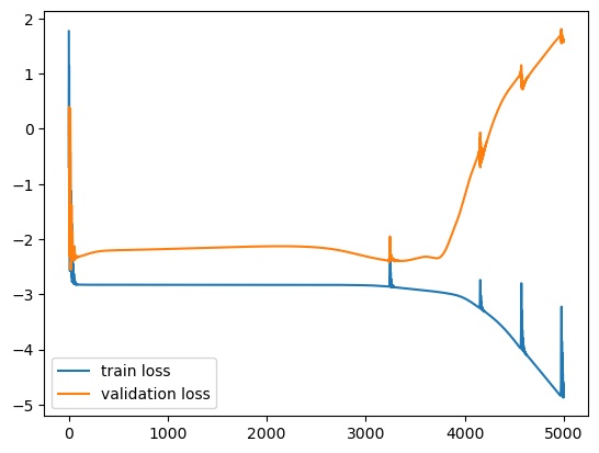
2.2 Detecting overfitting with validation

We are going to focus on the large model, but this time, we will perform validation at the end of each epoch.

large_model = MLP(hidden_dim=1024, num_hidden_layers=8)

optimizer = optim.Adam(large_model.parameters())
num_epochs = 5000

losses = {
    'val_loss': [],
    'train_loss': [],
}

with trange(num_epochs) as progress:
    for epoch in progress:
        train_loss = F.mse_loss(large_model(xs_train), target_train)
        optimizer.zero_grad()
        train_loss.backward()
        optimizer.step()
        
        # validation
        with torch.no_grad():
            val_loss = F.mse_loss(large_model(xs_val), target_val)
        
        train_loss = train_loss.detach().item()
        val_loss = val_loss.item()
        
        losses['train_loss'].append(train_loss)
        losses['val_loss'].append(val_loss)
        progress.display(
            'train_loss=%.4f, val_loss=%.4f' % (train_loss, val_loss))

df = pd.DataFrame(losses)
df.head()

	val_loss	train_loss
0	0.883441	5.854383
1	0.977545	0.491185
2	1.484757	3.012334
3	0.676571	3.106008
4	0.099790	1.453448

pyplot.plot(df.index, np.log(df.train_loss))
pyplot.plot(df.index, np.log(df.val_loss))
pyplot.legend(['train loss', 'validation loss']);